SATI is a spatial and spectral imaging Fabry-Perot interferometer in which the etalon is a narrow band interference filter and the detector is a CCD camera. SATI is an instrument adapted to measure the column emission rate and vertically averaged rotational temperature of the O2 atmospheric (0-1) band (layer centred in 94 km of altitude and the OH Meinel (6-2) band (layer centred in 87 km of altitude) as well as gravity waves which goes through these layers.
 |
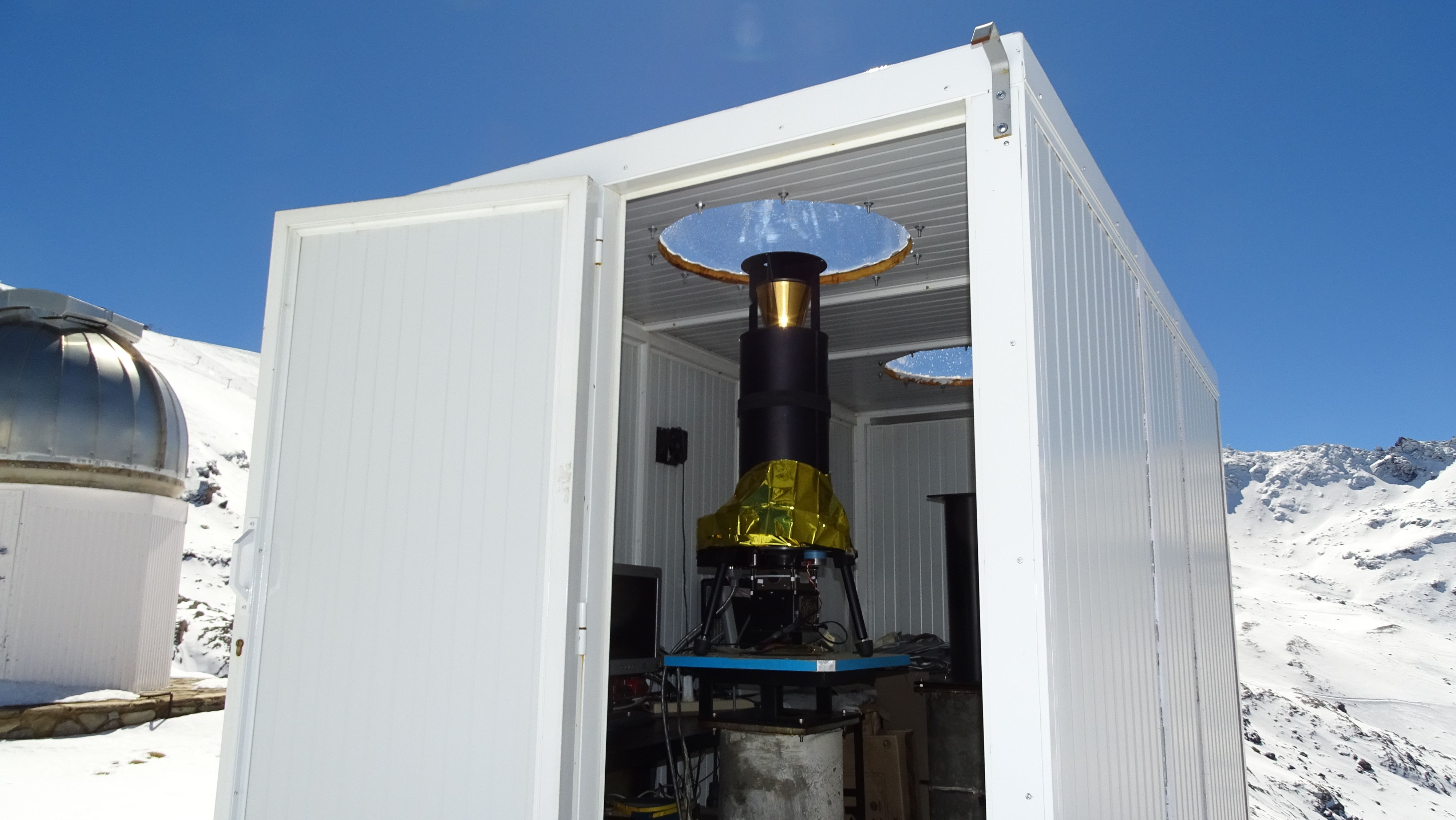
| Figure 1: Instrument |
SATI was installed at Sierra Nevada Observatory (37.060N,3.380W), Granada, Spain, at 2896 m of altitude. It has been continuously working since October 1998. The analysis of SATI measurements gives important information on:
- Behaviour and variability of the airglow emission rates of the O2 atmospheric (0-1) band and the OH Meinel (6-2) band.
- Behaviour and variability of the atmospheric temperature of this region.
- Dynamic and variability of this atmospheric region.
Instrument
The field of view produced by the conical mirror of 15o of semiangle and the baffles, is a cone centred to 30o from optical axis with an angular half-width of 7.1o. Thus, an annulus of average radius of 55 km and 16 km width at 95 km of altitude (or an average radius of 49 km and 14 km width at 85 km) is observed on the sky. SATI uses two interference filters, one centred at 867.689 nm (in the spectral region of the O2 atmospheric (0-1) band) and the second one centred at 836.813 nm (in the spectral region of the OH Meinel (6-2) band).
| Interferential filter | Central Wavelenght | Bandwidth |
| O2 filter | 867.689 nm | 0.231 nm |
| OH filter | 836.813 nm | 0.182 nm |
An interference filter, centred at λ0, and having a refractive index μ, ransmits the spectral lines of increasing wavelength, at decreasing incidence angles according to the equation:

Then a spectral line at wavelength λ, is trasmited an angle θ on the CCD. The images are disks where the azimuth dimension corresponds to the azimuth of the ring of the sky observed, while the radial distribution of the images contains the spectral distribution, from which the rotational temperature is inferred.
The images obtained from SATI can be analyzed as a whole, obtaining an average of the rotational temperature and emission rate of the airglow band from the whole sky ring; this allows a good monitoring of the behaviour of rotational temperature and emission rate for long periods of time, or by dividing the images in different sectors obtaining information of rotational temperatures and emission rates of each sector of the sky ring, from which the horizontal velocity of a disturbance can be determined.
(0-1) band of the O2 atmospheric system
 |
| Figure 2: Synthetic spectrum of the (0-1) O2 atmospheric band |
Figure 2 shows a synthetic spectrum of the (0-1) band of O2 atmospheric system. The magnetic dipolar transition b1Σ+g - X3Σ-g consists in doubles P Q branches: PP, PQ, RR and RQ. The PP and PQ branches of the spectrum of the O2 atmospheric (0-1) band appear as pairs of lines of 0.13 nm separation, and these pairs are separated from each other by 0.32 nm. These lines pairs in convolution with the 0.230nm bandpass of the interference O2 filter appear as single lines. The RR and RQ Branches at wavelength shorter than 864.5 nm are also pairs of lines but the separations beweeten these pairs are shorter and can not be solved as individual rings (see figure 3).
Figure 3 shows a typical image obtained with SATI by using the O2 filter. An integration time of 120 s has been used to obtain this image. The six rings correspond to the pairs of PP and PQ lines corresponding to the transitions K=3, 5, 7, 9, 11 and 13.
 |
| Figura 3: SATI image obtained by using the O2 interferential filter. |
(6-2) OH Meinel band
 |
| Figura 4: Spectrum synthetic of the OH (6-2) Meinel band. |
Figure 4 shows a synthetic spectrum of the OH(6-2) Meinel band. This band consists of P, Q and R branches. The line pairs of the R branch are mixed among them and the separation between them is very short to resolve them spectrally. The first three pairs of lines of the Q branch of the OH (6-2) Meinel band appear as pairs of lines (Q1q1, Q2q2 y Q3q3) of a separation from 0.1 to 0.3 nm, and these pairs are separated from each other by about 0.7 nm. These line pairs in convolution with the 0.182 nm bandpass of the interference filter produce two single lines corresponding to the transition K=1 and K=2; the pair of lines corresponding to the transition K=3 appears as two single rings and one of which, q3, is of extremely low emission rate.
Figure 5 shows a typical SATI image obtained by using the OH interferential filter with a integration time of 120 seconds.
 |
| Figura 5: SATI image obtained using the OH interferential filter. |
Images
 |
 |
| Figures 6 and 7: Lineal transformations of O2 and OH SATI images. | |
To obtain the spectrum we need to know the position on the CCD of the ring centre, the wavelength of maximum filter transmission, λ, and the effective index of refraction, μ, of the filter. Once the centre is determined the angular radius of each pixel is obtained. The radial variation of the signal of the SATI image obtained are shown in figures 6 and 7. The radial dimension is changed to wavelength dimension and then the spectral distribution of the signal is obtained (see figures 8 and 9).
 |
 |
| Figura 8: O2 spectrum from the O2 SATI image |
Figure 9: OH spectrum obtained from the OH SATI image. |
Emission rates and temperature
We use modelled spectra, spesynthetic(λ), to find the spectrum that best fits the observed spectrum, spemeasured(λ). The modelled O2 and OH spectra, spesynthetic(λ), are obtained by convolving the pure emission spectrum with the finite passband of the O2 and OH interference filter. The observed spectrum, spemeasured(λ), is the result of multiplying this normalized spectrum, spesynthetic(λ), by some factor, A, and adding a spectrally constant background, B. A least squares solution of the equation:

for all the radial points from radii 20 to radii 115 provides a estimation of the unknown A and B for each spectrum at the assumed temperature. A library of 150 synthetic spectra, for temperatures between 1100K to 2600K, is used in the least squares fitting.
The fitting is performed for each spectrum, and the one that yields the minimum fitting error gives its temperature value, T, the emission rate, A, and the continuum background, B.
Atmospheric Dynamic
The necessity of long term programs of observing airglow emissions from low, middle and high latitudes is a requirement to know the global behaviour of these emissions and also the behaviour of different atmospheric parameters, including temperature and chemical constituents. Data are needed to understand the chemical and dynamical processes that are producing the seasonal tendencies observed at different latitudes. In this sense data from SATI of emission rates and rotational temperatures will be added to other sets of data obtained at similar latitudes together with other sets of data coming from lower and higher latitudes, with the object of making a global study to understand the processes that are producing the variabilities detected in the upper atmosphere. The analysis of the temporal behaviour of these emessions let us to detect the presence of different atmospheric waves: planetary waves, tides and gravity waves. The analysis of these waves in terms of periods, amplitudes, phases and ocurrence allow us to obtain a valuable information about the atmospheric dynamic of this region.
The IAA is participating in the Network for the Detection of Mesopause Change (NDMC) with SATI measurements. The NDMC is a global program with the mission to promote international cooperation among research groups investigating the mesopause region.
 |
| Figure 10: Seasonal behaviour of monthly temperatures. |